Pharmacokinetics and Pharmacodynamics Crash Course + Cheat Sheet

Pharmacokinetics and pharmacodynamics are the cornerstones of pharmacology. Studying them together helps to paint a clearer picture of the safety and efficacy of a new drug. These studies are often performed as part of the pre-clinical trials in the drug development process. In this crash course, we cover the essential concepts in basic pharmacokinetics and pharmacodynamics and how to apply them, along with a cheat sheet with all the important formulas.

Pharmacokinetics: What the Body Does to the Drug

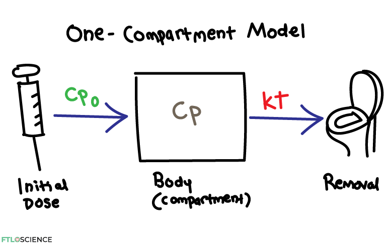
Skipping ahead of patient variations and ADME and bioavailability—all of which are still important, by the way—at the core of pharmacokinetics is studying what the body does to the drug. When a drug is administered to a patient, it enters their bloodstream. At this point, concentration is at its maximum (Cp0). The body quickly gets to work breaking it down and removing it from the body, helped by metabolic processes like the cytochrome P450 family of enzymes.

First Order Kinetics

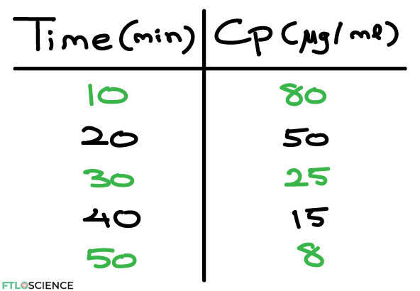
A simple way to model these processes all at once is to measure the blood plasma concentration (Cp) of the drug over a period (t). This is done by taking blood samples from the patient at various times after administration. A typical data set will look something like this:

If we plot this in a scatter graph, this is the result:

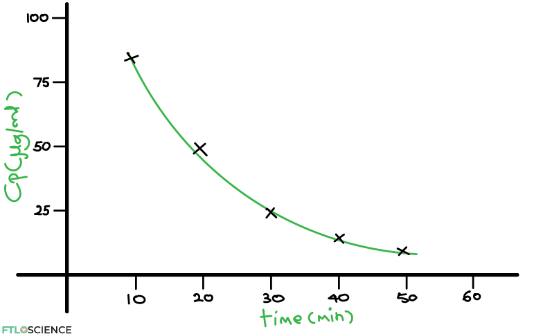
The key takeaway is that we see an exponential decay, which just means that the more drug there is in the body, the faster it’s removed. As time passes, the rate of decrease slows down. Many biological processes follow an exponential decay such as this; in pharmacokinetics, we say that such drugs follow first-order elimination kinetics.

(Note: because first-order kinetics are the most studied, we will focus on it in this crash course. Equations for zero-order and second-order kinetics are still provided in the cheat sheet at the end)

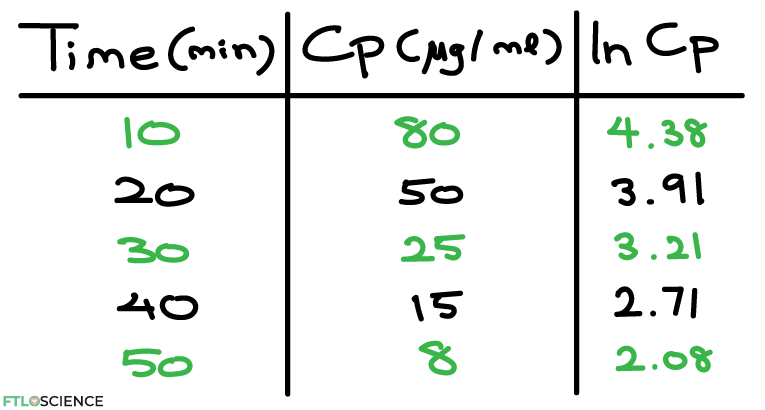
If we want more information about the drug, we can convert the exponential curve to a straight line. We first convert the Cp values to ln Cp (natural log), then plot those values.:

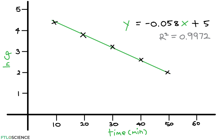
From the plot, we can now produce a line of best fit through the points. The equation of the line is given as:

y=-0.058x \:+ \:5

The One-Compartment Model

Why is this equation important? What we see above is the one-compartment model, where the maximum drug concentration (Cp0) exponentially decreases over time. This decrease is by the gradient of the straight line (k), when we take the natural log of the concentration values.

Putting this into mathematical terms, we can write that:

Cp=Cp_{0}\:\ast \:e^{-kt}\\[0.1in]
or \\[0.1in]
ln \:Cp =ln\:Cp_{0}-kt

Where Cp is the concentration of drug, Cp0 is the initial concentration at the point of administration, t is time and k is the elimination first order rate constant. The bottom equation follows the same form as the equation of the straight line in the ln Cp vs time plot!

y=mx+ c\\[0.1in]
ln \:Cp =-kt+ln\:Cp_{0}\\[0.1in]
\:y=ln \:Cp\:| \:  m=-k\:|\:x=t\:|\:c=ln\:Cp_{0}

The initial concentration of the drug is Cp0, which is given as the intercept c in the straight line. This means we can now calculate the initial concentration (when t = 0), something that is physically impossible to measure!

When \:t=0,\\[0.1in]
ln \:Cp =ln\:Cp_{0}\\[0.1in]
ln\:Cp_{0}=c=5\\[0.1in]
Cp_{0}=e^{c}=e^{5}=148.4\:\mu g/ml

Another useful relationship we have established is that changing the sign of the gradient of the graph (m) gives us the elimination rate constant (k).

The Elimination Rate Constant (k)

This constant k is useful because it allows us to calculate pharmacokinetic parameters, such as clearance (CL). Clearance is the volume of blood that gets cleared of the drug as a result of our metabolism, measured in L/hr or ml/min.

CL=k\:\ast\:Vd

The volume of distribution (Vd) is the apparent volume in which the drug is diffused throughout the body. Water-soluble drugs usually have a high Vd, while lipid-soluble drugs have a lower Vd. It is measured by taking the dose of the drug (X0) and dividing it by the maximum concentration (Cp0)

Vd = \frac{X_{0}}{Cp_{0}}

Half-life (t_1/2)

In pharmacokinetic studies, it can be useful to know the half-life of a drug, or the time it takes for its concentration to decrease by half in a patient. The half-life (t_1/2) of a drug that follows first-order kinetics can be calculated by this equation:

t_{1/2}=\frac{0.693}{k}

This is interesting because it tells us that the drug’s half-life depends only on its rate constant (k) and not its concentration!

Pharmacodynamics: What the Drug Does to the Body

While pharmacokinetics studies the change in drug concentration, pharmacodynamics deals with the observed effects of the drug on the body. Although drug concentration plays a role in pharmacodynamics, drug effects change from patient to patient. Differences in the biological makeup and genetics often make drug effects difficult to predict.

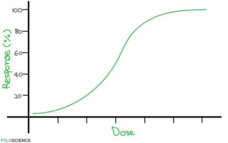
The drug’s effect and dose are often plotted to establish an initial relationship. The ‘effect’ should ideally be an easily measured change caused by the drug. Different dosages are administered to test subjects so that a dose-response curve can be plotted. Below is an example of a dose-response curve.

Effective, Toxic, Lethal Dose Values

Dose-response curves can be used to predict effective, toxic and lethal doses of a specific drug, depending on the response. For example, if we want to study efficacy, we can test the response in certain receptors on a piece of tissue. If we want to test for toxic and lethal doses, we can use live animals to study the drug’s effects. Pre-clinical studies such as these are a key part of the drug development process.

ED_x (effective dose): the drug dose that will cause a therapeutic effect in x% of the population

TD_x (toxic dose): the drug dose that will cause toxic effects in x% of the population

LD_x (lethal dose): the dose that will be lethal to x% of a population.

In an ideal drug, its ED₅₀ value should be much lower than the TD₅₀ and LD₅₀ values. This means that it can be dosed at therapeutic levels without risking the patient’s safety. A drug that has ED50 = LD10, for example, would not be very safe!

Therapeutic Window of a Drug

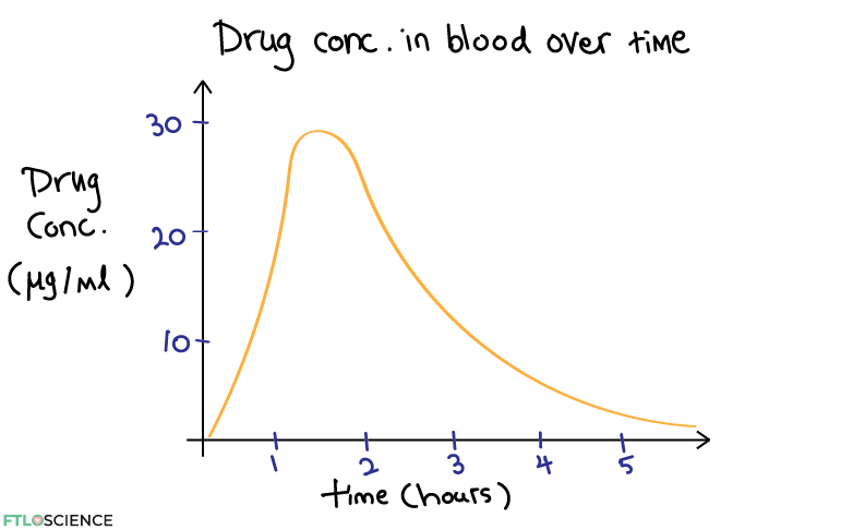
Once we establish the effective and toxic concentrations of the drug, we can combine this with the information from the drug plasma concentration over time studies. A typical profile of drug plasma concentration over time has a distinct rapid rise in concentration followed by a slow decrease as the drug is metabolized and eliminated from the body.

Let’s say we have found from dose-response studies that 1) the drug is only effective at a concentration of 10 μg/ml and 2) it starts to show toxic side effects at 20 μg/ml. We can now create an overlay for the concentration over time plot:

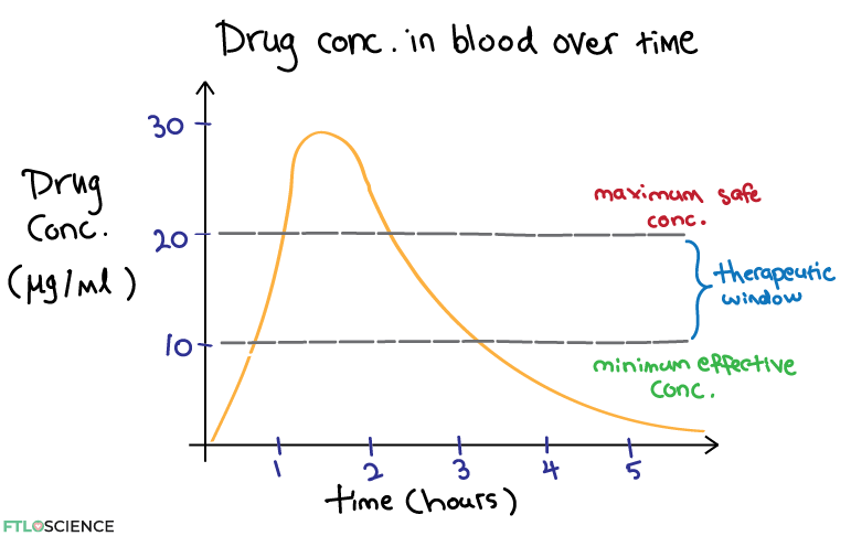
Below the minimum effective concentration threshold, the drug is ineffective. Above the maximum safe concentration, the drug causes adverse reactions. The ‘sweet spot’ between these two limits is the therapeutic window. Pharmacodynamic studies such as these help us to better understand the ideal dosage of a new drug to recommend for patients.

Therapeutic Index (TI)

To quantify the safety of a drug, its therapeutic index (TI) can be measured, where:

TI = TD_{50}/ED_{50}

A drug with TI >> 1 will be safer than a drug with a drug that has a TI close to 1, since it will have a bigger therapeutic window between the toxic dose and the effective dose.

Pharmacokinetics and Pharmacodynamics Cheat Sheet

First-Order Kinetics

Cp=Cp_{0}\:\ast \:e^{-kt}\\[0.1in]
ln \:Cp =ln\:Cp_{0}-kt\\[0.1in]

In a straight line plot:

y=mx+ c\\[0.1in]
\:y=ln \:Cp\:| \:  m=-k\:|\:x=t\:|\:c=ln\:Cp_{0}

If plotting software is not used, the gradient of the line (m) can be calculated by:

m = \frac{∆y}{∆x} = \frac{y_{2} \:– \:y_{1}}{ x_{2}\: –\: x_{1} }

Half life (t_1/2)

t_{1/2}=\frac{0.693}{k}

Zero-Order Kinetics

General equation and half-life equation:

Cp = Cp_{0} -kt\\[0.1in]
t_{1/2} = \frac{Cp_{0}}{2k}

Second-Order Kinetics

General equation and half-life equation:

\frac{1}{Cp} = \frac{1}{Cp_{0}} + kt\\[0.1in]
t_{1/2} = \frac{1}{k\ast Cp0}

Other Useful Equations

Vd = \frac{X_{0}}{Cp_{0}}\\[0.1in]
CL = k \ast Vd\\[0.1in]
TI = \frac{TD_{50}}{ED_{50}}

Glossary of Terms and Units

Cp: drug plasma concentration (μg/ml or mg/L)
Cp0: maximum drug plasma concentration (t=0)
CL: clearance (ml/min or L/h)
k: elimination rate constant (min^-1 or hr^-1)
t_1/2: Half-life, time taken for drug concentration to be halved (min or hr)
Vd: Volume of distribution (L)
ED_x: the drug dose that will cause a therapeutic effect in x% of the population (μg or mg or g)
TD_x: the drug dose that will cause toxic effects in x% of the population (μg or mg or g)
LD_x: the dose that will be lethal to x% of a population (μg or mg or g)
TI: a measure of drug safety, TI >> 1 = safe, TI close to 1 = unsafe